Table of content

• 1/ How should I organize my workplace before every single analysis?
• 2/ How Should I run my analysis?
• 3/ How segmentation models have been generated?
• 4/ How segmentation models have been validated?
• 5/ Should I use Generalist or Specialist Model for Mitochondria Segmentation?
• 6/ How to determine the diameter to use to segment mitochondria?
• 7/ Can I use another software beside Cellpose to segment mitochondria?
• 8/ Does EM magnification modify mitochondrial measurements?
• 9/ Does EM magnification affect mitochondrial segmentation accuracy?
• 10/ Does image quality/contrast affect mitochondrial segmentation accuracy?
• 11/ How do I know that the segmentation is satisfactory?
• 12/ What is a Neural Network?
• 13/ What is a Confusion Matrix?
• 14/ How do I read/interpret a confusion matrix?
• 15/ What is a Shapley Additive exPlantions?
• 16/ How do I read/interpret a Shapley Value plot ?
• 17/ What is Spatial Clustering?
• 18/ ERROR MESSAGE

1/ How should I organize my workplace before every single analysis?

BEFORE the ANALYSIS:

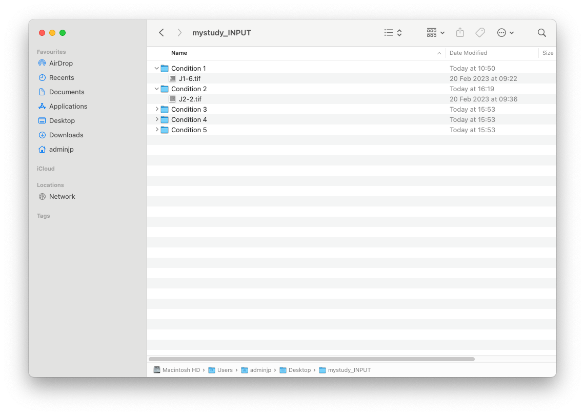
1/Create an INPUT folder. We suggest the following name “mystudy_INPUT”

This input folder must contain as many folders as you have conditions to compare. For example, if you have one group of “Wild Type”, you may create a subfolder called “Wild_type”. This folder must contain all EM images generated from your wild type samples, and anything other.

Please be advised that the name of each condition will be used and displayed in the different output generated from computation modules (Data display, and data prediction).

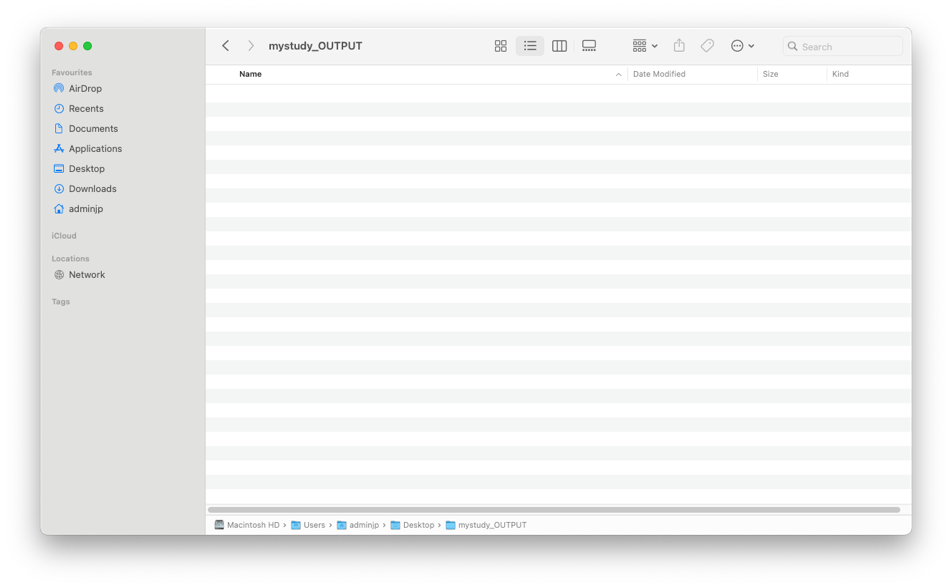
2/Create an OUTPUT folder. We suggest the following name “mystudy_OUTPUT”

️Before EACH Analysis, this folder MUST be EMPTY️. Otherwise, EMITOMETRIX will not be able to run.

DURING the ANALYSIS:

️In any case, DO NOT MODIFY any of the folders/files created in the OUTPUT folder️

AFTER the ANALYSIS:

1/In the OUTPUT Folder, as soon as the step 1 (Segmentation) has started, 9 folders are automatically created

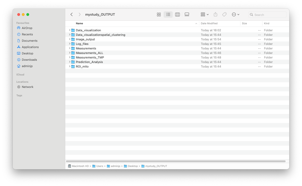
2/Each folder will contain specific informations. For example in the “Data_visualization” folder you will find all emitometrics graph, with one color per condition.

3/ Once the full analysis is done, you can archive all images from the INPUT folder and all files from the OUTPUT folder in a safe place

NB: for more detailed instructions, please go to the instructions manual (link)

2/ How Should I run my analysis?

• STEP1: SEGMENTATION

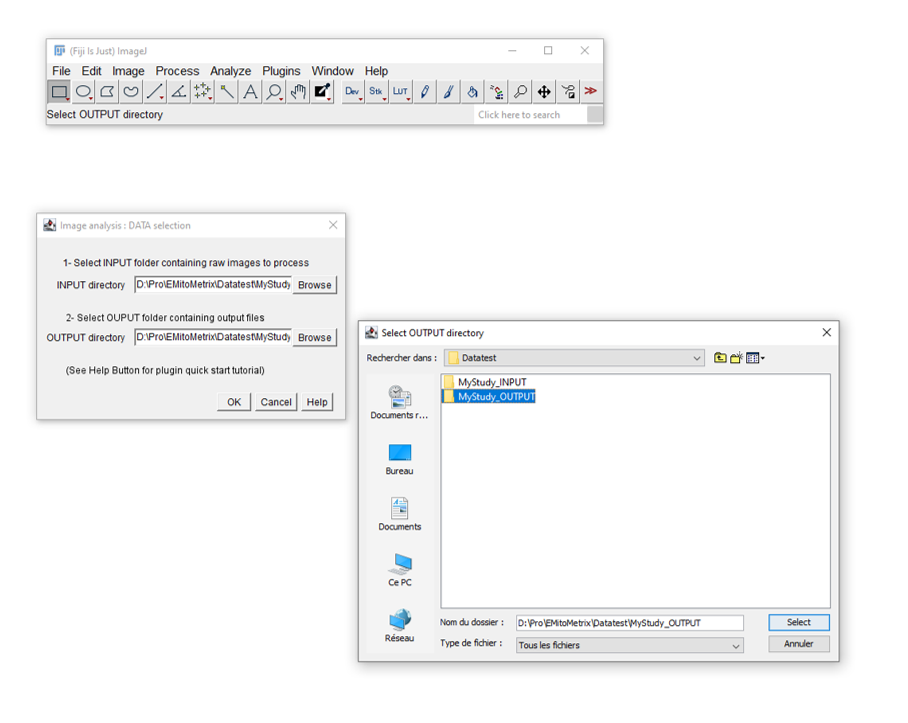
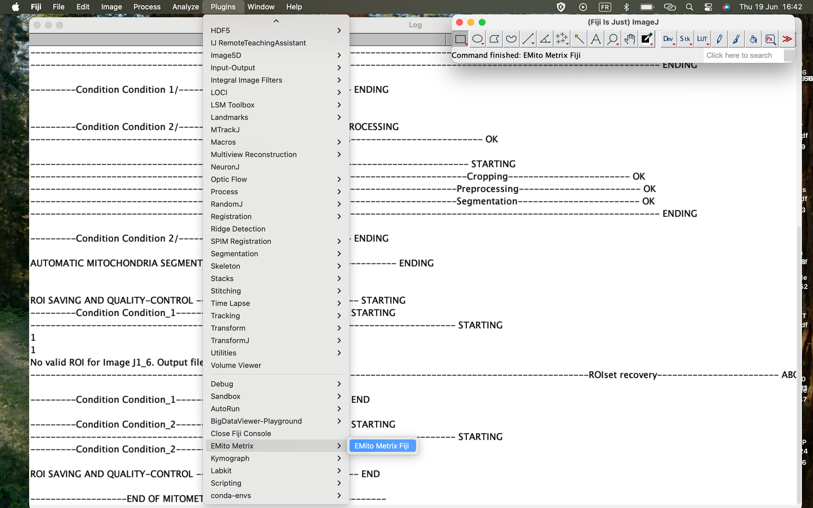
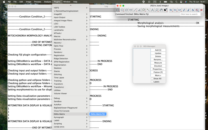
• Double click on the FIJI icon, then go to Plugins>EmitoMetrix
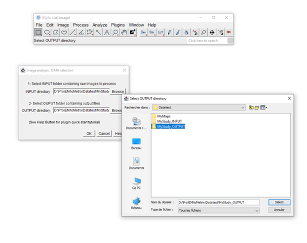
• Please indicate the path of your INPUT and OUTPUT FOLDERS

• Follow down the dialog boxes
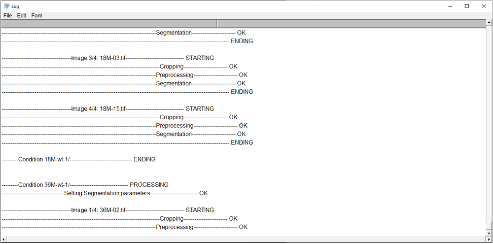
• Then STEP1 is starting, that may take a lot of time. You will be able to follow the processing on the “LOG” Window.

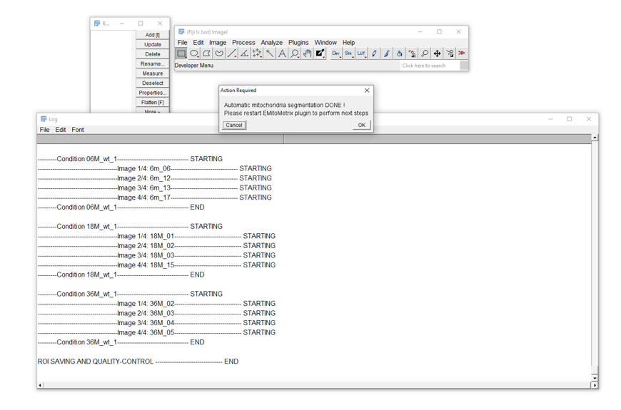
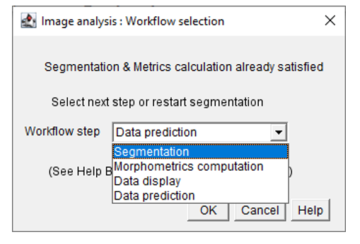
• Once the segmentation is done, the user will see this dialog box, and will be able to move on to the next step.

• STEP2: MITO-METRICS CALCULATION:

• To launch the STEP2, please go to Plugins>EmitoMetrix

• Please indicate the path of your INPUT and OUTPUT FOLDER
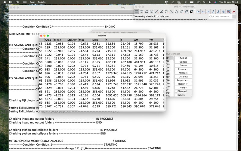
• Calculations will then start image per image and condition per condition

• Once mitometrics calculation is done, the user will see this dialog box, and will be able to move on to the next step.

• STEP3: DATA-DISPLAY:

• To launch the STEP3, please go to Plugins>EmitoMetrix
• Please indicate the path of your INPUT and OUTPUT FOLDERS
• Follow down the dialog boxes to set up the metrics and the style of every graph you would like to generate.

• Once data display is done, the user will see this dialog box, and will be able to move on to the next step. All graphs will then be found in the OUTPUT folder.

• STEP4: DATA COMPUTATION/PREDICTION:

• To launch the STEP4, please go to Plugins>EmitoMetrix

• Please indicate the path of your INPUT and OUTPUT FOLDER
• Follow down the dialog boxes to set up the ML model you want to try
• Then STEP4 is starting, that may take a lot of time. You will be able to follow the processing on the “LOG” Window.

• Once data computation is done, the user will see this dialog box, and will be able to move on to the next step.

3/How segmentation models have been generated?

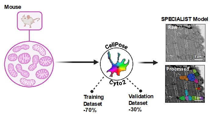
Training of the various Species-specific and Generalist models was carried out using Cellpose 2.0 software.. For each specie, the images acquired by TEM were randomly separated into 2 distinct groups, one - training dataset (70%) - used for training each model, and the second - validation dataset (30%) - for model validation. For each image of the training group, mitochondria were first detected using the Cyto2 model implemented in Cellpose. To fine-tune the Cyto2 model with our images, we used Cellpose 2.0's Human-in-the-loop training function and manually annotated, one by one, mitochondria not detected or partially detected by the Cyto2 model (False Negative). For each image, we also took care to remove all false detections (False Positive). Thus, correctly annotated, these images were used in the Cellpose 2.0 software to fine-tune the initial model (Cyto2) and generate our own models.

• >Example of one Specialist Model: Mouse_SM: 652 images and 32032 mitochondria were manually annotated out of Skeletal Muscle (Soleus, Gastrocnemius, Quadriceps), Heart, or Liver.

For the Specie-Specific Models SM:

• Worm-Specific model: training was carried out on 344 images, for a total of 3533 annotated mitochondria.
• Drosophila-specific model: training was carried out on 11 images, for a total of 965

annotated mitochondria.

• For the Z-Fish-specific model: we used 249 images and manually annotated 11668 mitochondria
• For the K-Fish-specific model: we used 155 images and manually annotated 5125 mitochondria
• For the Fish-specific model: we used 404 images and manually annotated 16793 mitochondria
• For the Mouse-specific model, 652 images and 32032 mitochondria were manually annotated.
• For Human-specific model, 39 images and 2391 mitochondria were manually annotated.

• For the Generalist model (GM), we combined images and annotations from the 6 Species-specific models, for a total of 809 images and 25895 mitochondria manually annotated.

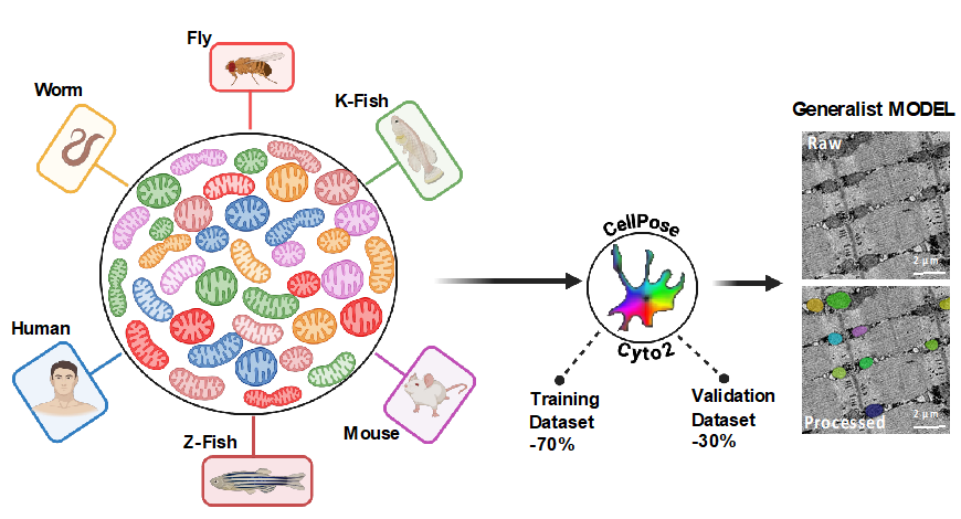
• >The Generalist Model_GM: Model was finetuned using images and annotations from the 6 Species-specific models, for a total of 809 images and 25895 mitochondria manually annotated.

4/ How segmentation models have been validated?

Each of the 7 trained models was then validated using different images from the validation group (175, 10, 107, 67, 174, 297, 17 and 346 images, respectively for Worm-specific, Drosophila-specific, Zebrafish-specific, Killifish-Specific, Fish-Specific, Mouse-Specific, Human-Specific and Generalist. Using Cellpose 2.0 software, we subjected each image to its 2 corresponding models - Species-specific and Generalist - and obtained a mitochondrial segmentation prediction map (P) for each. In parallel, for each validation image, we manually annotated the mitochondria to obtain a Ground Truth map (GT).

To assess the performance of the 7 Species-specific models and the Generalist model, we compared the prediction and ground truth maps for each mitochondrion, and measured various performance indicators using Fiji software:

- Intersection map (P ∩ GT): corresponds to the area of colocalization between a mitochondrion predicted by the model and its nearest ground truth (annotated mitochondrion)

- Union map (P ∪ GT): corresponds to the projection of a predicted mitochondrion and its nearest ground truth.

- Intersection over Union or IoU: corresponds to the ratio between intersection (P ∩ GT) and union (P ∪ GT). This score is calculated for each mitochondrion, and represents a measure of a model's accuracy for an object detection spot. Its value ranges from 0 to 1, with 1 for a perfect object prediction. Note that a score greater than 0.5 is considered by consensus to be the threshold value for good prediction.

For each image in the validation group, we then used these calculated IoU values to measure various performance metrics:

- True Positives TP: number of objects in the prediction map with an IoU value greater than 0.5. This metric corresponds to the number of mitochondria correctly predicted by the model.

- False Positive FP: number of objects in the prediction map with an IoU value less than or equal to 0.5. This metric corresponds to the number of erroneous predictions.

- False Negative FN: the number of mitochondria not predicted by the model. It corresponds to the difference between the number of ground-truth mitochondria and the number of true positives (GT - TP).

- Precision (TP / (TP+FP)). Indicates the extent to which the objects predicted by the model are real (i.e. are mitochondria). The calculated score ranges from 0 to 1.

- Sensitivity (TP / (TP+FN)). Indicates the model's ability to predict all or some of the real objects (mitochondria). The calculated score ranges from 0 to 1.

- Average Precision AP (TP / (TP+FP+FN)). Performance indicator that takes into account the 2 criteria of specificity and precision. The calculated score ranges from 0 to 1.

- DICE Score

For each trained model (species-Specific or Generalist), the mean Average Precision (mAP) is calculated by averaging the AP score calculated for each image in the validation group.

5/ Should I use Generalist or Specialist Model for Mitochondria Segmentation?

Each specie-specific model has been trained using images of the different tissues from single specie (i.e. ZebraFish, Mouse, Fly, Human, Killifish or C-Elegans). This implied that dataset used for each model training had a high homogeneity of tissue’s environment. On this opposite, we used images of skeletal muscle from several species (i.e. ZebraFish, Mouse, Killifish, C-Elegans and Human) to train our Generalist model, that is dataset with a very high heterogeneity of tissue’s environment. Because of this heterogeneity, and depending on the tissue and/or specie you use, you may have a better mitochondria detection using the Generalist model than the Species-specific models (see below).

• Projection of EM image of skeletal muscle biopsy (left panels) and liver biopsy (right panels) of Mice with mitochondria segmentation map (color-coded)*. For each tissue, we used either Generalist or Mice-specific model as an input for Cellpose mitochondria detection. The number of detection is indicated for each condition * Images from CBM (CSIC-UAM), UAM University - Laura Formentini

For better precision and sensitivity of detection, we recommend testing both Generalist and Specific models on your dataset, before starting EMitoMetrix application

We do not recommend using Cellpose trained models (cyto2, nucleus, cyto), as these models have not been trained on EM images.

6/ How to determine the diameter to use to segment mitochondria?

The Cellpose neural network used in our EMitoMetrix application has been separately trained on images from tissues and different species, resulting in so many different species-specific models. For each model, we annotated mitochondria with various diameter; however, using Cellpose neural network in an automatic way needs a user-defined mitochondria diameter (in pixel) as an input for segmentation.

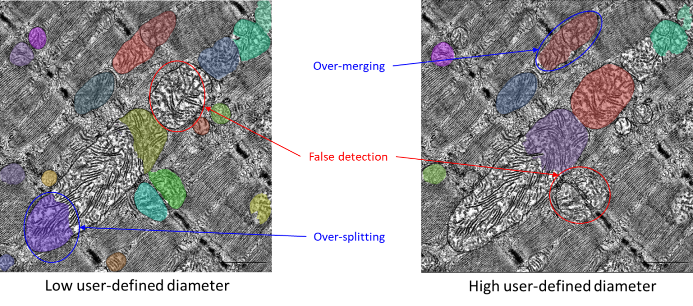
• Projection of EM image of skeletal muscle biopsy of Mouse with mitochondria segmentation map (color-coded)*. We used either a low value (left panel) or a high value as a user-defined diameter for mitochondria detection * Images from CBM (CSIC-UAM), UAM University - Laura Formentini.

User defines the size value as the average diameter of mitochondria from a single image, or from an image-by-image basis. Changing the diameter will change the results of the algorithm outputs (i.e. the objects segmented). When the diameter is set smaller than the true size, then the neural network model may over-split mitochondria. Similarly, if the diameter is set too big, then the neural network model may over-merge mitochondria. In the Emitometrix interface, user has to define a main diameter per image (or per condition). Therefore, if the tissue’s region imaged contains mitochondria with strong size heterogeneity (i.e. large and small mitochondria in the same image), the neural network model may detect mitochondria with a poor accuracy (for example an over-splitting of large mitochondria and/or an over-merging of small mitochondria, as shown below).

To overcome this issue, the user has the option to define a range of mitochondrial diameters (a minimum and a maximum value) in addition to the main value. This feature is optional, meaning that the user can choose to set only one value (either minimum or maximum), both, or neither.

• Setting mitochondria segmentation

In Cellpose window, drag and drop your input image to analyze. Here is an example of the Cellpose graphical interface and its functionalities:

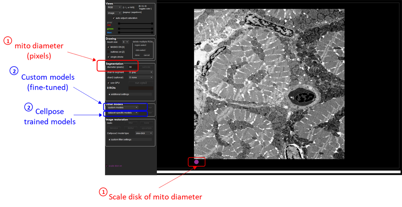
Using Cellpose application, estimate the following segmentation settings:

- Mitochondria size (in pixels): defined as the average diameter of mitochondria to detect in the image (see for more details about diameter definition)

Use the purple circle (at the bottom of the view) as a scale disk of the user-defined diameter value

- Trained model to use for automatic segmentation (see for more details)

You can choose either a Cellpose trained model (cyto2, nucleus, cyto) or one of our custom Generalist or Species-specific EM models.

Once you have set both diameter and trained model, click on the run button to check the mitochondria segmentation. Adjust diameter accordingly if the segmentation is not working.

Depending on mitochondria size heterogeneity of your dataset, you may need to set your diameter value by image, by condition (single value for all images of the condition) or by study (single value for all conditions)

For more details about Cellpose GUI instructions, please use this link

NB: There are also alternative options to calculate the average size of any ROI such as FIJI. This video tutorial here is quite helpful: FIJI (ImageJ): Regions of Interest and the ROI Manager: link to tutorial.

️️For Mac user️️, here is a simple pipeline to install and use Cell Pose:

0/ Install Anaconda to be able to run Python command line. The best is to follow carefully step by step this video tutorial

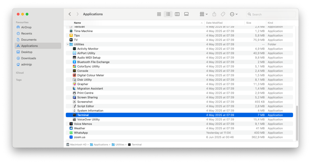
1/Launch the terminal using the finder>applications>Utilities>Terminal

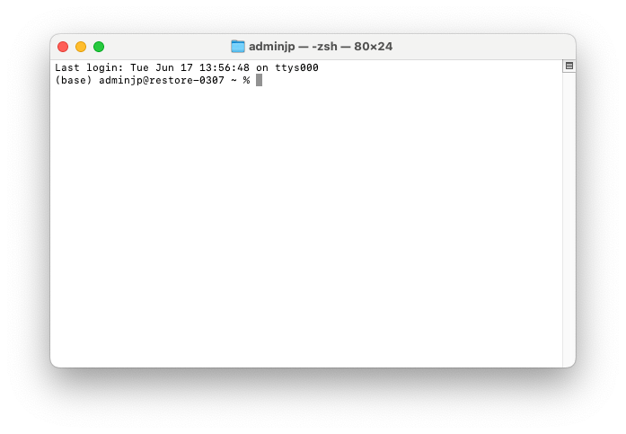
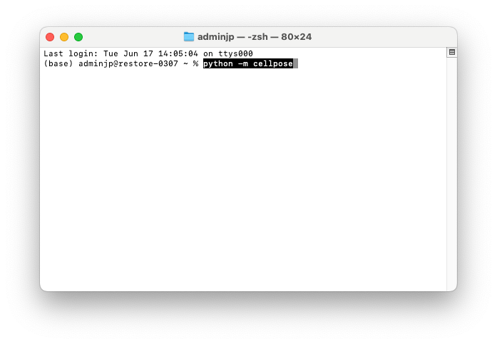
2/ Open the terminal by double clicking on the icon and this window should pop-up

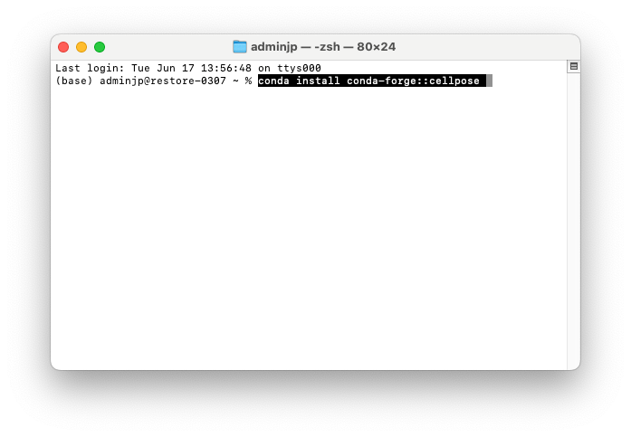
3/To install “CellPose” type this command line “conda install conda-forge: :cellpose”

4/Once installed, to launch the app type “python -m cellpose”

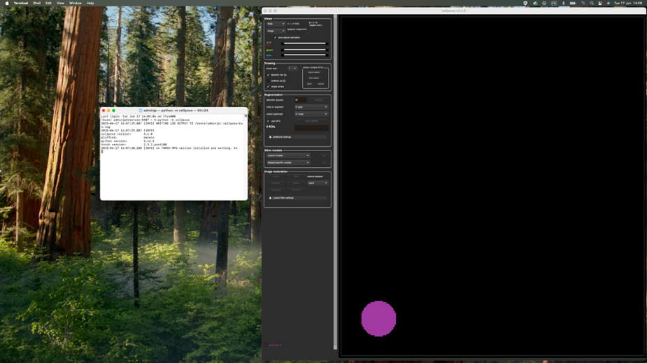
5/CellPose window should then pop-up as followed, you can drag any image in the app

NB: There are also alternative options to calculate the average size of any ROI such as FIJI. This video tutorial here is quite helpful: FIJI (ImageJ): Regions of Interest and the ROI Manager: tutorial.

7/ Can I use another software beside Cellpose to segment mitochondria?

We have added, in EMitoMetrix tool, the option for the user to import their own segmentation maps (segmentation performed outside of our pipeline, Empanada for example or with own-trained model), and putting back into the EMitoMetrix pipeline in order to perform data analysis, mitometrics visualization and data prediction. Here are the instructions to follow carefully to import and analyze your own segmentation maps in the EMitoMetrix tool: • Before starting the analysis, your data must be organized as follows:

1. An INPUT folder containing your raw TEM images (see here for more details).
2. An empty OUTPUT folder that will contain the output data.
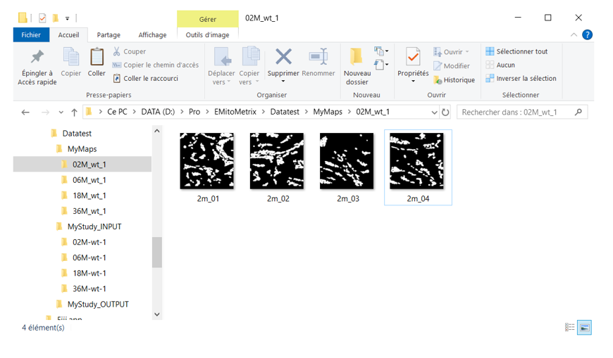
3. For each condition, a MAPS folder containing the segmentation maps. Each MAPS folder should contain the segmentation maps only. The filename of each map should match that of the corresponding raw image.

• From the Plugins menu in Fiji, launch EMitoMetrix.
• Please specify the INPUT folder containing your raw data and the OUTPUT folder.

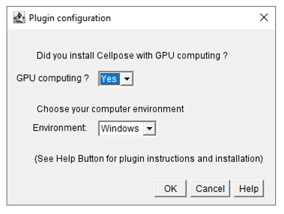
• Select the environment type (Windows, Linux, or MacOS) and the calculation mode.

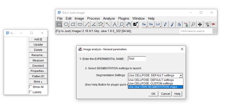
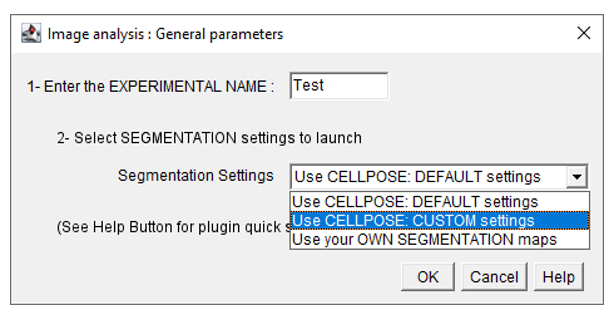
• In the general parameters window, select use your OWN SEGMENTATION maps from the segmentation settings menu.

• Fill in the parameters in the next windows (general and preprocessing settings).
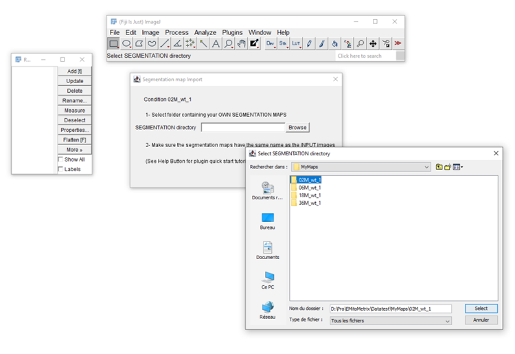
• For each condition, in the Segmentation map import window, please indicate the MAPS folder containing the segmentation maps. These segmentation maps will be copied into the corresponding Cellpose_mask folder in the OUTPUT/image_output directory.

• Once the import is done, the user will be able to restart EMitoMetrix to proceed to the next steps (analysis, data display, and data prediction).

8/ Does EM magnification modify mitochondrial measurements?

In electron microscopy (EM) mitochondrial analysis, panoramic images enable the visualization of the tissue but not the details of each mitochondrion. Larger images are useful for gaining finer mitochondria measurements, such as Cristae’s orientation, parallelism, and Cristae’s quantity within the mitochondria. In optical microscopy, the resolution of images is closely related to the magnification used during acquisition. The higher magnification, the greater resolution for morphology and ultrastructure details

Modifying magnification during the acquisition will affect the resolution of EM images, i.e. the resolution of mitochondrial features. Therefore, when running EMito-Metrix analysis, this magnification variation will result in variations of some mitochondrial measurements – especially morphological measurements -, as shown in the following figure.

If you plan to analyze and compare one-by-one several conditions, we highly recommend that you use the same magnification so that you can compare the corresponding morphological measurements.

9/ Does EM magnification affect mitochondrial segmentation accuracy?

While using a high magnification may be necessary to obtain high-resolution images of mitochondria, it is worth noting that precision and sensitivity of the model used for mitochondria segmentation is highly dependent on mitochondria’s environment, i.e. the type of tissue imaged (see below).

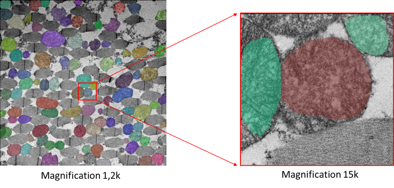
• EM image of the same skeletal muscle biopsy of Drosophila, acquired at magnification of 1.2k (left panel) or 15k (right panel). For each case, we have projected mitochondria segmentation on the raw EM image. We observe an erroneous segmentation from the 15k magnification, which is due to the absence of tissue’s context

When setting both magnification and tissue’s region to acquire, we recommended that you choose an area containing several mitochondria (at least 2 mitochondria) associated with their tissue environment. This should guarantee better mitochondria detection (see below).

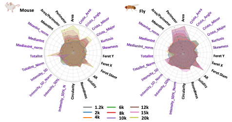
We tested if our fine-tuned GM model was working at high magnification. Specie per Specie, we compared mitochondria segmentation from 1,2k to 20k resolution. We found that mitochondria segmentation was working very well but with a variable accuracy depending on the specie. Thus, we established that our model works at maximum 15k images for Fly, 12k images for Z-Fish and 20k images for Mouse.

10/ Does image quality/contrast affect mitochondrial segmentation accuracy?

In conventional optical microscopy, the quality of the biological information contained within an image depends on multiple factors acting throughout the data lifecycle. It relies not only on the algorithms and procedures employed during the image processing and analysis stages but, more critically, on upstream steps such as sample preparation and image acquisition. Although numerous analytical tools currently enable restoration or correction of image intensities, a low-contrast or low-resolution image will yield poor-quality information, regardless of its nature (quantitative, morphological, or qualitative). This issue is particularly pronounced when attempting to identify and analyze the morphology of fine and highly resolute structures such as mitochondria. For these reasons, it appears essential for experimenters to rigorously control and validate a series of prerequisites during sample preparation and image acquisition prior to EMitoMetrix analysis, as discussed here (Culley S, et al., 2023).

For the training of all Specialist and Generalist models, we selected images acquired with different magnifications (from 1.2k to 20k). We ensured that each selected image had high-contrast and high-resolution, thus excluding images with a low signal-to-noise ratio. For all these reasons, the segmentation proposed in our EMitoMetrix tool may present certain reservations - regarding its precision and sensitivity - in two specific cases:

• using low-contrast or low-resolution images : difficulty to differentiate mitochondrial cristae from the background, or badly separating mitochondria close to each other.
• using images acquired with very high magnification (>15/20k): over-segmentation of mitochondria due to higher-resolute morphology/cristae than the one used for training, or insufficient tissue context (see here).

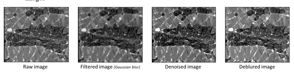
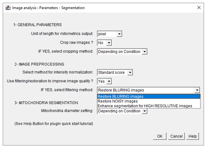
To partially correct for these limitations highly dependent on image quality, EMitoMetrix has been enhanced with three restoration/filter functionalities that enable users to correct images prior to segmentation:

• debluring which enable to restore low resolute images
• denoising which enable to restore images with low signal-to-noise ratio.
• Gaussian filter which enable to smooth image intensities, enhancing segmentation for higher resolute images

These functionalities are already implemented in the Cellpose 3.0 tool, as described here (Stringer C., et al. 2024).

Image Restoration/filtering is applied before image segmentation. If you would like to use these functionalities, please follow these instructions:

• From the Plugins menu in Fiji, launch EMitoMetrix.
• Specify the INPUT folder containing your raw data and the OUTPUT folder.
• Select the environment type (Windows, Linux, or MacOS) and the calculation mode.
• If you have already done both image segmentation and analysis, please select Segmentation in the Workflow selection window

• In the general parameters window, select use CELLPOSE: CUSTOM settings from the segmentation settings menu.

• Fill in the following parameters in the Image preprocessing menu : set use filter/restoration menu to Yes, and select the appropriate filtering method from the following menu :

• Fill in the parameters in the next windows. Once the segmentation is done, the user will be able to restart EMitoMetrix to proceed to the next steps (analysis, data display, and data prediction).

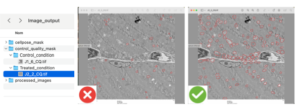
11/ How do I know that the segmentation is satisfactory?

EMito-Metrix offered two options to help the users to determine is the mitochondria segmentation is satisfactory.

Option 1:

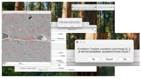
Once the segmentation is run after the first step, every single image processed by the interface will pop-up, and by visually checking the quality of the mitochondria segmentation, the user will be able to either include the image by clicking “Yes” or the exclude the image by clicking “No”. All images excluded during this step, will not be included for the mitochondria metrics calculation during the next step.

Option 2:

If needed, afterwards the user will be able to access to all images with mitochondria segmentation. In the OUTPUT folder, in the the “image_output” folder>“control_quality_mask” > “xyz_condition”.

If the segmentation is not satisfactory, few extra rounds of optimization would be required, notably on the average size of the mitochondria. We recommend to pick one or two images per condition, and test a broad range of “size” and pick the best one (see section 3).

11/ Which are the prediction models of Machine Learning available in EMito-Metrix?

Two different classes of machine learning algorithms have been employed: tree-based models (Random Forest, LR parser and XGBoost), and a neural network (MultiLayer Perceptron, MLP). We split the dataset into training and test datasets (80% and 20% respectively) and we compared the performance of each algorithm in terms of good prediction (Accuracy score).

Youtube link for tutorial video : All Machine Learning algorithms explained

• Tree based algorithms:

Tree-based algorithms are a fundamental component of machine learning, offering intuitive decision-making processes akin to human reasoning. These algorithms construct decision trees, where each branch represents a decision based on features, ultimately leading to a prediction or classification.

Source: geeksforgeeks - tree based machine learning algorithm

• Neural Network:

Neural networks are machine learning models that mimic the complex functions of the human brain. These models consist of interconnected nodes or neurons that process data, learn patterns, and enable tasks such as pattern recognition and decision-making.

Source: geeksforgeeks - neural network a beginners guide

13/ What is a Confusion Matrix?

Machine Learning involves feeding an algorithm with data so that it can learn to perform a specific task on its own. In classification problems, it predicts outcomes that need to be compared to the ground truth to measure its performance. The confusion matrix, also known as a contingency table, is commonly used for this purpose. It not only highlights correct and incorrect predictions but also provides insights into the types of errors made. To calculate a confusion matrix, you need a test dataset and a validation dataset containing the actual result values (Source:Datascientest.com ).

Youtube link for a video tutorial:What is a Confusion Matrix?

14/ How do I read/interpret a confusion matrix?

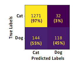
In this example: we have asked the ML models to predict the proportion of cats or dogs on every single image of a given dataset. The results are displayed using a confusion matrix as shown here. How to read it? At first, on the left side are laid out the “True labels” which is the ground truth, and on this dataset, there are 1303 (1271+32) cats and 262 (144+118) dogs. Then, the models will predict and label each animal from image as cats or dogs, and the results are shown at the bottom of the matrix with the “Predicted labels”. In our example, out of 1303 cats contained in our image, 1271 have been rightly classified by the ML model as “cat” and 32 have been erroneously classified as “Dog”, leading to 97% of right prediction (1271/1303*100) and 3% (32/1303*100) of wrong prediction (False negative). Similarly, out of 262 dogs, 118 have been rightly classified as “Dog” and 144 have been erroneously classified by the model as “Cat”, leading to 45% of right prediction (118/262*100) and 55% (144/262*100) of wrong prediction (False negative). The accuracy score indicated on top of the matrix is the sum of right predictions (1271+118)/ all predictions (1271+32+144+118)= 88,7%.

15/ What is a Shapley Additive exPlantions?

SHapley Additive exPlanations, more commonly known as SHAP, is used to explain the output of Machine Learning models. It is based on Shapley values, which use game theory to assign credit for a model’s prediction to each feature or feature value. (Source:datascientest.com ).

16/ How do I read/interpret a Shapley Value plot ?

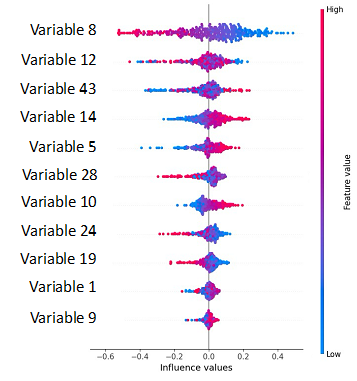
As stated earlier, SHapley Additive exPlanations, more commonly known as SHAP, is used to explain the output of Machine Learning models and to compute the contribution of each feature to the prediction of each instance, for the model. The contributions are then aggregated on a single plot to identify the contribution of each feature at a glance.

In this example let’s assume we have asked our model to predict out of an image dataset whether it is a cat or a dog. You see that out a large number of variables (over 50) only 11 are shown on the plot and those are the strongest variable, which have helped the model to make its prediction “it is a cat”. Now, all the variables are ranked in the order of importance in the prediction from top to bottom. Variable 8 is number one on the list (on the top), implying that this feature is the one with the highest contribution in the model. Additionally, the color scale on the right handside indicates whether it is a low value (blue) or a high value (red) that contributes to predict positively (right side-“it is a cat”) or negatively (left side-“it is not a cat”). In our example low values of variable 8 lead to predict positively the outcome, and high values of the variable 8 lead to a negative prediction “it is not a cat”.

17/ What is Spatial Clustering?

• Spatial Clustering is an option available during STEP3, that enable on all pictures from any conditions to identify spatial clustering.

• Please be advised that running this option will drastically slow down the processing and the overall step 3.
• For all images, spatial clustering results will be available in the OUTPUT folder “Data_Visualization_SpatialClustering”

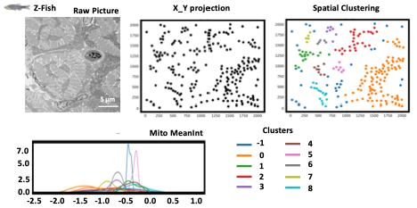
• For each dataset, and for each picture the user will have acces to X/Y projection where all black dots are the segmented mitochondria (from STEP1) displayed on the image based on their X/Y coordinates.
• Then, on this X_Y projection, a Spatial clustering it is applied, where mitochondria “groups” are identified using one different color per cluster.
• It is possible to get all mitometrics, and have them display cluster per cluster like MeanInt as shown on the example here.

18/ ERROR MESSAGE

• Checking FIJI plugin configuration --------------------------- ERROR

  This message appears if one or more Fiji plugins (Cellpose-BIOP & Bio-Format) are missing. To solve this issue, please install these plugins from the Fiji’s help menu.

• Checking input and output folders --------------------------- ERROR

  Invalid folders are detected from the INPUT directory (Missing folders containing input images, for example). Please see the FAQ for input instructions.
  Invalid folders are detected from the OUTPUT directory. Please see the FAQ for input instructions.

• Checking python and cellpose folders --------------------------- ERROR

  Invalid Python folder or missing files. Please see the FAQ for installation instructions.
  Invalid Cellpose environment or Cellpose folder. Please see the FAQ for installation instructions.

• Setting Data visualization parameters --------------------------- ERROR

  User must select at least 3 or more Morphology & texture metrics for data display. Please see the FAQ for instructions.

• Setting Morphology Analysis parameters --------------------------- ERROR

  User must select at least 1 or more graph or data distribution to display. Please see the FAQ for instructions.

• Setting Mitochondria Segmentation parameters --------------------------- ERROR

  An invalid value has been set for Mitochondria Diameter (cellpose segmentation). An integer value (higher than 0) has to be set. Please see the FAQ for segmentation settings.

• Setting Data computation parameters --------------------------- ERROR

  No machine learning model has been selected for data prediction. Please see the FAQ for instructions.

• Checking mitochondria diameter for segmentation

  An invalid value has been set for Mitochondria Diameter (cellpose segmentation). An integer value (higher than 0) has to be set. Please see the FAQ for segmentation settings.

• Setting Mitochondria Segmentation parameters --------------------------- ERROR

  INPUT folder contains one or more images with invalid file format. Please convert input images using conventional format (TIF).

18/ WARNING MESSAGE

• Checking image format for segmentation

  File format WARNING: File format selected (jpeg or jpg) has poor resolution compared to conventional format (TIFF). This can lead to lower quality results.

• Checking for Data display settings

  WARNING: Selecting Spatial clustering during data display step will increase calculation time.

• Checking for Data computation settings

  WARNING: Computing the explanation for MLP model will substantially increase calculation time.

• Checking for General settings

  Warning: Allowing image display during analysis will slow down macro execution.

• Checking ROI for morphological analysis

  No valid mitochondria ROI has been detected during segmentation step, for the image. Image not included for the three next steps.

• Checking folder for segmentation

  A non-valid condition folder has been detected in the INPUT directory. Folder not included for the three next steps.

• Checking folder name for segmentation

  A non-valid folder’s name has been detected in the INPUT directory (wrong characters). Folder not included for the three next steps. Please stop the analysis and rename the folder if necessary.

• Checking folder content for segmentation

  An empty folder has been detected in the INPUT directory (no input images). Folder not included for the three next steps.

• Checking image name for segmentation

  A non-valid image’s name has been detected in the INPUT directory (wrong characters). Image not included for the three next steps. Please stop the analysis and rename the image if necessary.